Why Your Extended Kalman Filter Diverges at Highway Speed

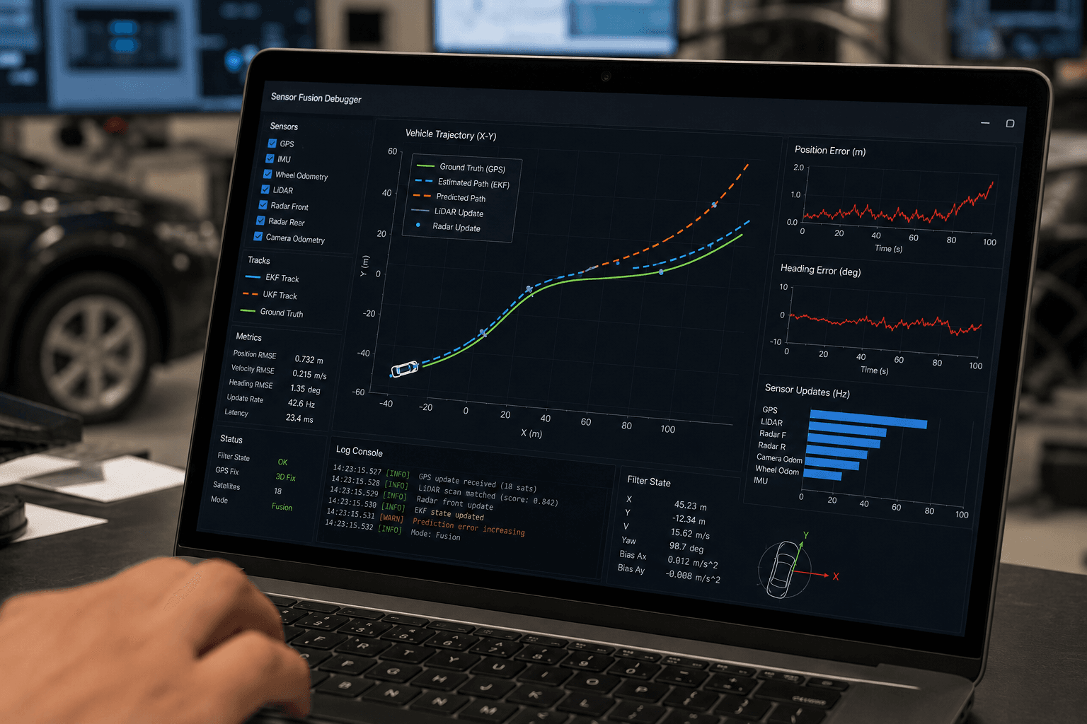
Process noise tuning matters more than your motion model. Here is the math and the fix.

Every EKF-based tracker we've shipped has passed the same first test: slow-speed, low-density scenarios — parking lots, campus roads, 20-30 km/h — where the filter tracks smoothly and the innovation stays tight around zero. And nearly every one of them has, at some point, failed the same second test: put the same vehicle on a highway at 100+ km/h, and the track quality falls apart. Not immediately, not catastrophically at first — just a slow, then sudden, divergence where the filter's estimate walks further and further from the sensor measurements until it's effectively tracking noise.

This is a specific, well-understood failure mode, and it's worth writing down properly because the instinct most engineers have when they see it — "the motion model must be wrong" — is usually not where the bug actually lives.

The Setup: Fine at 30 km/h, Broken at 100 km/h

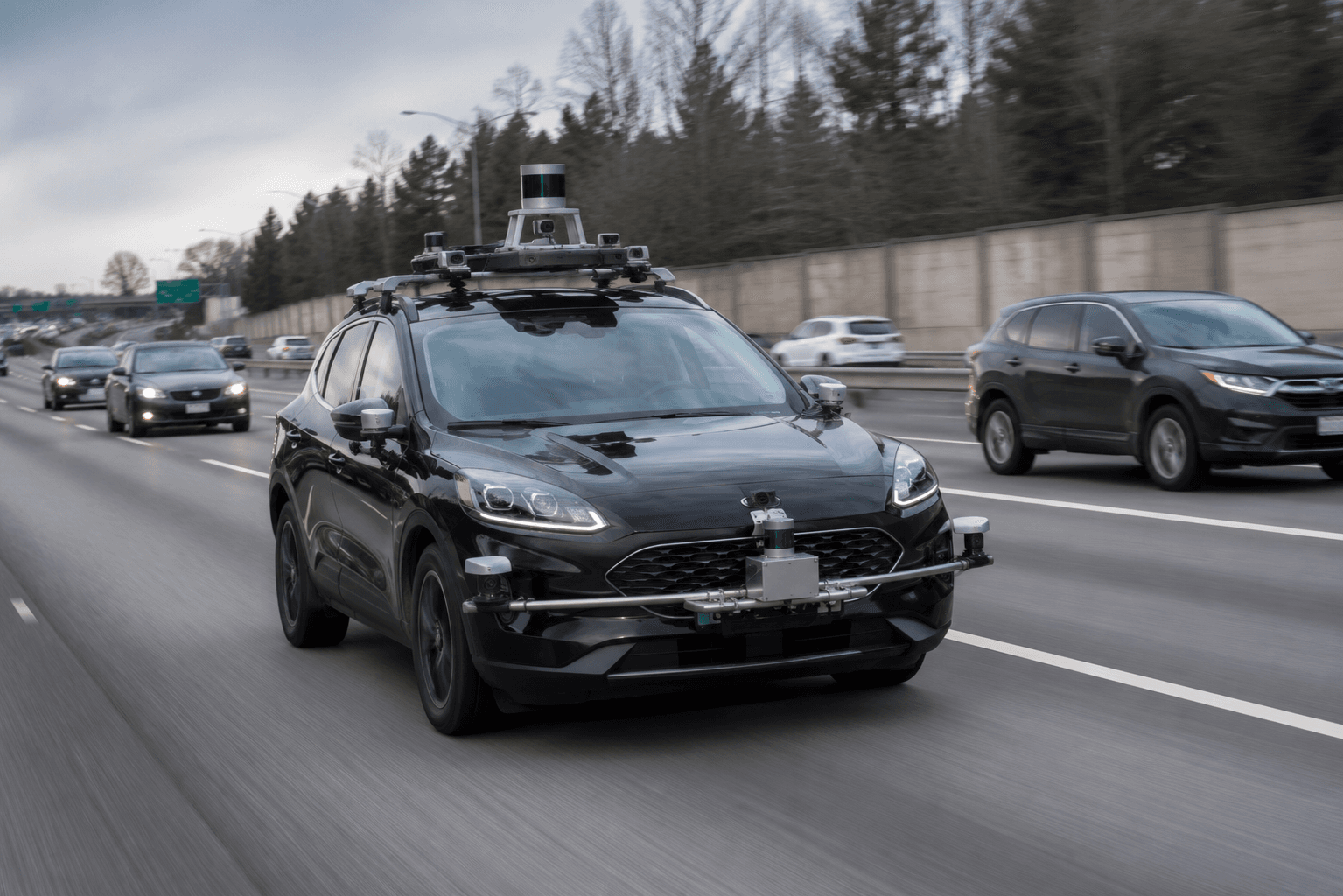
Our target tracker used a standard constant-turn-rate-and-velocity (CTRV) motion model in an EKF, fusing radar range/range-rate with camera bounding box centroids. In closed-course testing at low speed, tracking a lead vehicle through gentle curves, the filter behaved exactly as expected — smooth state estimates, tight covariance, innovation sequences that looked like white noise centered on zero.

The moment we moved to highway testing, tracking vehicles at relative speeds well above 100 km/h with occasional hard braking events from the lead car, we started seeing tracks that would hold for a few seconds and then visibly lag behind or overshoot the true target position — sometimes losing the target's actual position by more than a car length before the filter "caught up," and occasionally not catching up at all before track loss.

The natural first hypothesis on a team is always the motion model: is CTRV insufficient? Do we need a more sophisticated model with jerk terms? We spent the better part of a week going down that path before the data told us otherwise.

The Real Culprit: A Mistuned Q Matrix

The process noise covariance matrix, Q, encodes how much uncertainty the filter should inject into its own prediction at every timestep — essentially, how much the filter should distrust its own motion model versus trusting incoming measurements. Q had been tuned during low-speed testing, where target accelerations were modest and the CTRV model's linearization error was small. It was never re-validated at highway closing speeds.

Here's the part that's easy to miss: Q doesn't just need to scale with your uncertainty about acceleration — it needs to scale with how wrong your linearization is, and linearization error itself grows with speed.

The EKF linearizes the (generally nonlinear) motion model around the current state estimate at every timestep, using the Jacobian F. For CTRV, this Jacobian's off-diagonal terms — which couple velocity, heading, and turn rate — grow in magnitude as speed increases. A first-order Taylor expansion that's an excellent local approximation at 8 m/s can be a poor one at 30 m/s, particularly during a maneuver like braking or a lane change, where the true trajectory curves away from the linear approximation faster than the model accounts for.

A Q tuned to be "small" (because it worked at low speed, where actual approximation error was small) starts systematically underestimating the true uncertainty the moment the vehicle profile changes. The filter becomes overconfident in a prediction that is, in fact, increasingly wrong.

The Math, Briefly

The standard EKF prediction step propagates state and covariance as:

x_k|k-1 = f(x_k-1|k-1)
P_k|k-1 = F_k · P_k-1|k-1 · F_k^T + Q_k

where F_k is the Jacobian of the motion model f() evaluated at the current estimate, and Q_k is process noise.

The innovation (residual between prediction and measurement) is:

y_k = z_k − h(x_k|k-1)
S_k = H_k · P_k|k-1 · H_k^T + R_k

If Q_k is too small relative to the actual prediction error introduced by linearization, then P_k|k-1 understates true uncertainty, S_k becomes overconfident, and the Kalman gain K_k = P_k|k-1 · H_k^T · S_k^-1 shrinks — the filter trusts its own (wrong) prediction more than it should and discounts the measurement that would have corrected it. This is exactly backwards from what you want when the model is under stress, and it's a self-reinforcing failure: once the estimate starts drifting, the linearization is being evaluated at an increasingly wrong point, which makes the next prediction step even less accurate, while the (still too-small) Q keeps the filter confidently wrong.

This is the mechanistic reason process noise tuning matters more than motion model sophistication in this specific failure: you can have the "correct" nonlinear model and still diverge if Q doesn't account for how much your linearization degrades as the operating point moves away from where you tuned it.

Debugging It: Innovation and NIS

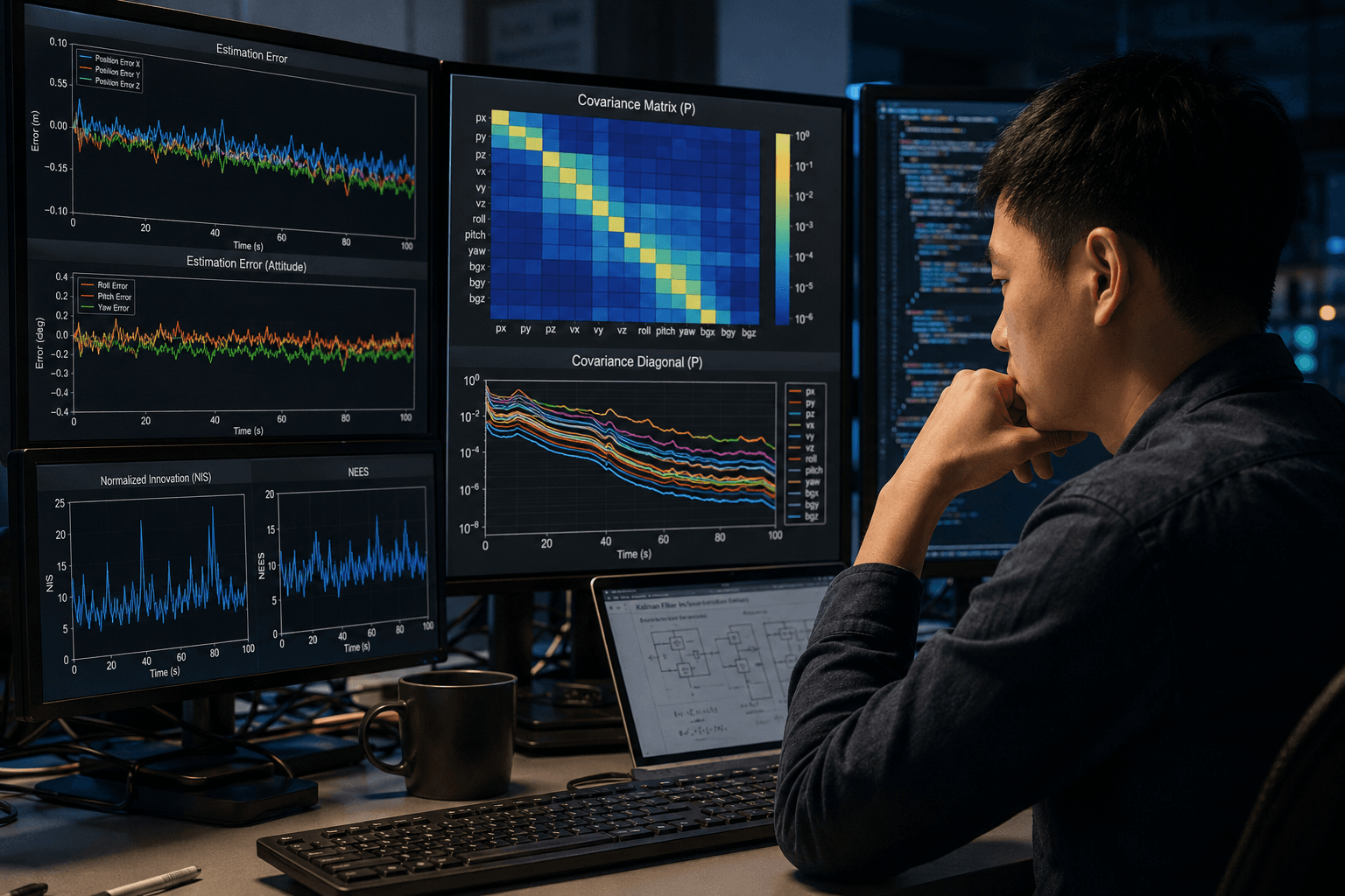
The diagnostic tool for exactly this situation is the Normalized Innovation Squared (NIS):

NIS_k = y_k^T · S_k^-1 · y_k

For a correctly tuned filter, NIS follows a chi-squared distribution with degrees of freedom equal to the measurement dimension. For a 2D position measurement, that's chi-squared with 2 DOF, with an expected value of 2 and a 95% consistency bound of roughly 5.99.

When we plotted NIS over time for our highway test runs, low-speed segments sat comfortably under the bound, averaging close to the expected value. High-speed segments told a completely different story: NIS climbing steadily above the 95% bound for sustained stretches, spiking dramatically during braking events. That's a filter that is, statistically, no longer consistent — its own covariance no longer reflects its actual error, which is precisely the signature of an undertuned Q.

We also plotted raw innovation directly against speed and lateral/longitudinal acceleration. The correlation was clean: innovation magnitude tracked closely with target acceleration magnitude, not with absolute speed itself — which pointed specifically at maneuvering (and the linearization error that comes with it) rather than speed as a raw scalar being the driver.

The Fix: Adaptive Q, and When to Reach for UKF

We implemented two changes, and validated each independently before combining them.

1. Speed- and maneuver-adaptive Q. Instead of a fixed Q tuned once, we scaled the acceleration-noise terms of Q as a function of estimated target dynamics — using a simple scheduled approach where Q scales up when recent innovation or estimated turn rate exceeds a threshold, functioning as a lightweight adaptive filter (a simplified relative of Sage-Husa or innovation-based adaptive estimation). This alone brought NIS back under the 95% bound for the large majority of highway test segments, including braking events.

2. Selective use of UKF for high-dynamics segments. For scenarios with sustained high nonlinearity — hard cornering combined with high closing speed — we moved to an Unscented Kalman Filter, which propagates a set of sigma points through the true nonlinear model rather than linearizing it. UKF doesn't eliminate the need for correct Q tuning, but it removes linearization error as a separate source of degradation, which made the remaining Q-tuning problem much easier to reason about and solve independently.

The combination — adaptive Q as the general-purpose fix, UKF reserved for the highest-nonlinearity operating regions where the extra computational cost was justified — resolved the divergence across our full highway test matrix, with NIS remaining within the consistency bound across more than 40 recorded highway sessions spanning speeds from 60 to 130 km/h.

The Lesson

The uncomfortable truth in this class of bug is that your filter can look completely correct in the test conditions you validated it in, and be fundamentally miscalibrated the moment operating conditions change — and the failure won't announce itself as a crash or an obvious error. It shows up as a slow, statistically detectable drift that's easy to dismiss as "sensor noise" if you're not specifically checking filter consistency.

A few things worth taking away:

Tune process noise across the full speed and maneuver envelope you expect to operate in, not just the envelope that's convenient to test. Low-speed, low-dynamics testing will always look fine with an undertuned Q — that's exactly the condition where linearization error is smallest.

NIS is not optional instrumentation — it should be a standing metric in every fusion validation run, the same way you'd never ship a classifier without a confusion matrix. A filter that's statistically inconsistent will eventually diverge somewhere, even if your current test scenario doesn't happen to trigger it.

A more sophisticated motion model is not automatically the answer to a divergence problem. We nearly spent a sprint building a higher-order motion model before the innovation data made it clear the actual problem was uncertainty calibration, not model structure. Check Q and NIS before you rearchitect the filter.

If your fusion stack is showing intermittent tracking drift that only appears at certain speeds or during aggressive maneuvers, it's worth plotting NIS before you touch the motion model — the data usually tells you which one is actually broken.